Phase-Based Video Motion Processing
Fork me on GitHub.
Many phenomena in real-life occurs at minuscule scales that are not perceptible with bare eyes, for instance, the swinging of skyscrapers due to winds, the pulsing change in skin color due to blood flow, or the wiggling of another person's eyes. The goal of video motion processing is to magnify such barely noticeable motions that are present in recorded videos. In this project, we reproduced the phased-based video motion processing algorithm proposed in the SIGGRAPH 2013 "Phase based video motion processing" paper (Wadhwa et al. 2013).
Results
The following are two results produced with our implementation (not all functionalities introduced in Wadhwa et al. 2013 are implemented).
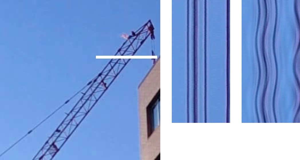
75x (correction) magnification of motions at 0.2–0.25Hz using a half-octave pyramid with 3 levels and 8 orientations.
25x magnification of motions at 72–92Hz using a half-octave pyramid with 3 levels and 8 orientations.
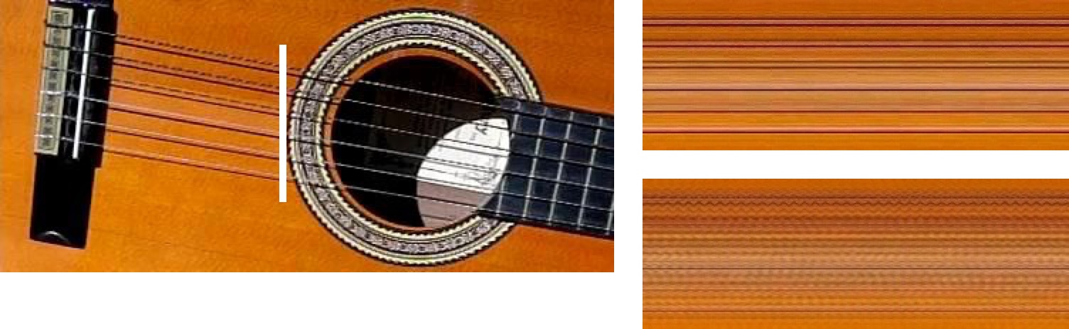
The processing was done in CIELAB color space on each channel separately. Each frame of the input video was decomposed into a complex steerable half-octave pyramid with 3 levels and 8 orientations. Motions at a specific frequency range are isolated with a band-pass FIR window temporal filter. It took approximately 10 minutes to generate each video using an Intel i9-9900K with 32GB memory.
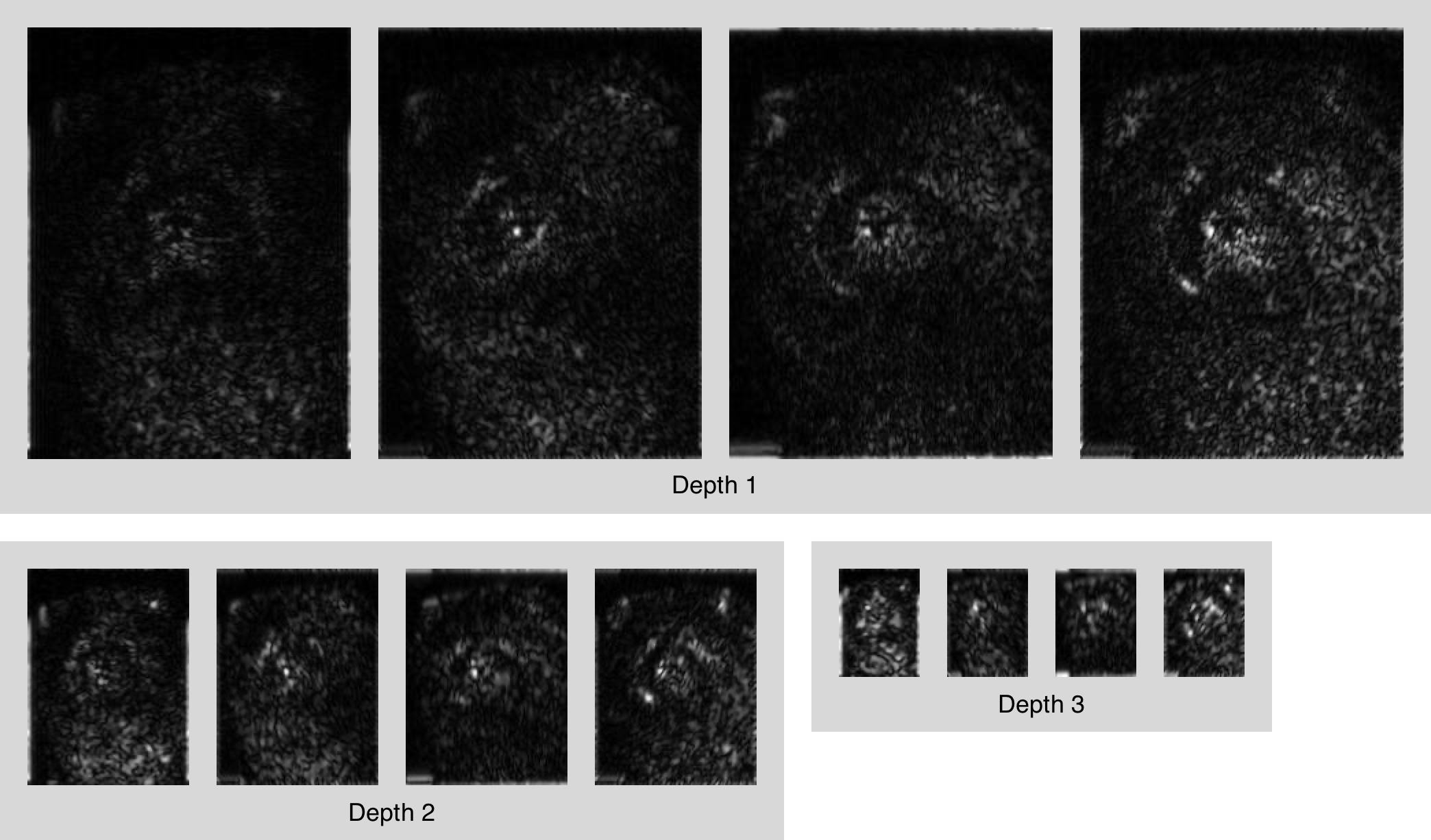
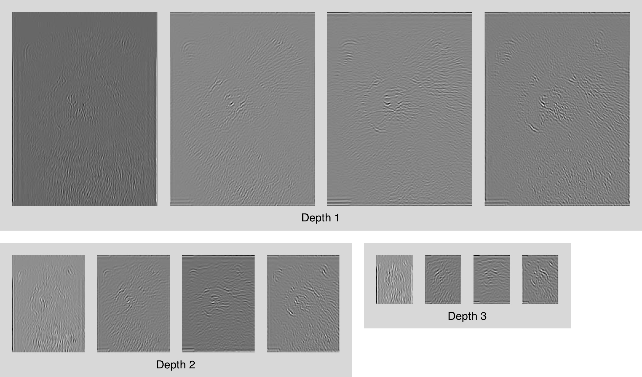
Complex Steerable Pyramid
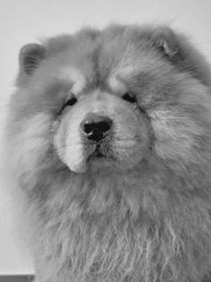
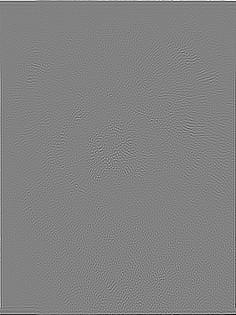
The following is a sample result of complex pyramid decomposition from our implementation.

Summary
The motivation for phase-based video motion processing comes from the Fourier shift theorem. Therefore, understanding the motion processing method used in this paper requires knowledge of Fourier analysis (cf. Wadhwa et al. 2013, Sec. 3).
We first represent an image with the Fourier synthesis formula. Let \(f\in\mathbb{R}^{[0,1]}\) denote a 1D image of unit length, where its values can be interpreted as luminance, then it can be written as a trigonometric polynomial using the definition of Fourier series, i.e.
\[f(x) = \sum_{k=-\infty}^\infty c_k \exp\left(i2\pi kx\right), \]
where \(c_k\) is some complex number.
Motion and Phase
The Fourier shift theorem states that
\[f(x+\delta(t)) = \sum_{k=-\infty}^\infty c_k \exp\left(i2\pi k(x+\delta(t))\right),\]
meaning that if the image is translated by \(\delta(t)\) over time, then it will appear as a phase shift on the trigonometric polynomial. If we take the phase component of \(f(x+\delta(t))\), and use a temporal filter with zero DC response to filter out the changing phase that corresponds to the translation, i.e. to extract
\[\Delta\phi(t)=2\pi k \delta(t),\]
then we can directly magnify or attenuate this translation by increasing or decreasing the change in phase via multiplication, i.e.
\[f'(x+\delta(t)) = \sum_{k=-\infty}^\infty c_k \exp\left(i2\pi k(x+\delta(t))\right)\cdot \exp\left(i\alpha\Delta\phi(t)\right),\]
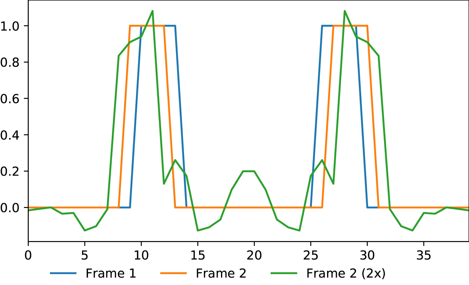
with \(\alpha > 1\) resulting in magnification and \(\alpha < 1\) in attenuation. Refer to docs/examples.ipynb for toy examples of motion modification.
However, most interesting motions are not just translations. Usually, motions are localized and we have to deal with \(\delta(x,t)\). Also, they would also require multiple frequency bands to represent, meaning that by indexing the motions by \(j\), we need to treat the phases over frequency bands \(k\in A_j\) as a whole. Now the motion is written as
\[f(x+\delta(x,t)) = \sum_j \left(\sum_{k\in A_j} c_k \exp\left(i2\pi kx\right) \right)\cdot \exp \left(i2\pi \sum_{k\in A_j} \delta_j(x,t,k)\right) ,\]
and we process each summand as a whose with temporal filters of appropriate pass-bands to isolate the motion of interest.
Complex Steerable Pyramid
Without further assumption, a simple method to partition the 2D frequency spectrum for motion extraction is the steerable pyramid. Ideally, the pyramid divides the 2D frequency domain into concentric rings and sectors of equal angles (cf. Wadhwa et al. 2013, Fig. 4).
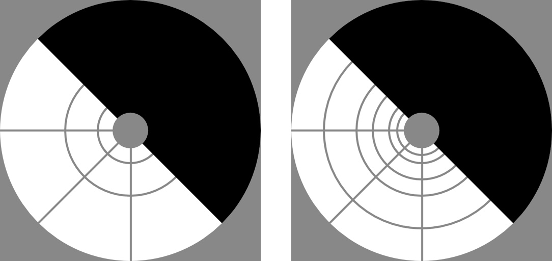
The corners comprise the high-pass residual, and the center part is the low-pass residual. The black conjugate symmetric portion is discarded.
Each partition captures objects of a certain size and orientation, hence motions of a certain scale and direction. The corners not included in the circle is the high-pass residual, and the center part that the pyramid of finite depth left un-partitioned is the low-pass residual.
Since for real-valued images, Fourier coefficients are conjugate symmetric, so we only need to keep half of the 2D frequency spectrum to perform processing on. On the other hand, we have to throw out the other half anyways, because the sum of each partition and its conjugate reflection gives a real-valued time-domain signal without the zero phase. This gives the "complex" nature of this pyramid.
Finally, note that as analyzed in (Wadhwa et al. 2013, Sec. 3.2), there is a trade-off between the amount of motion magnification that can be achieved, which means using a pyramid with more levels and orientations, and the amount of distortion in the output, which is minimized when using a pyramid with fewer levels and orientations.
Implementation Details
First, an overview is provided. As pictorially described in (Wadhwa et al. 2013, Fig. 2):
- Compute the complex steerable pyramid for each frame of the video (processed on \((x,y)\)-planes, where the video sequence lies on \((x,y,t)\)-hyperplane; now the changes in the phase component over time corresponds to motion). [details]
- Perform band-pass temporal filtering on the phase component of each image in the pyramid to isolate motion at specific frequencies (processed on \(t\)-axis, and now the amplitude of the resulting "image" corresponds to the amount of motion). [details]
- Smooth the "images" (omitted).
- Multiply the resulting "images" by \(\alpha\), and add it back to the phase component of the respective frames in the pyramid (positive coefficient gives motion magnification, and negative gives attenuation). [details]
- Reconstruct video by collapsing the pyramid. [details]
Algorithm (Motion Modification).
Input:
- \(I_{1:T}\) is a real-valued video sequence.
- \(D,K,N\) represents the depth, number of orientations and number of filters per octave to be used to construct the complex steerable pyramid.
- \(f_s\) represents the sampling rate of the video sequence, and \(f_l,f_h\) represents the frequency range of the motion to be modified.
- \(\alpha\) is the magnification factor.
- \(B,F\) represent the types of filters to be used to construct the pyramid and for temporal filtering, respectively.
Initialize:
- \(P_{1:T}\), \({R_H}_{1:T}\), \({R_L}_{1:T}\) represent the pyramid sequence.
- \(Q_{1:T}\) represents the pyramid for storing motion magnified frames.
- \(J_{1:T}\) is the output video sequence.
- Filter \(F\) with \(f_s,f_h,f_l\) as described in temporal filtering section.
For \(t=1,\cdots, T\), set \((P_t,{R_H}_t,{R_L}_t) \gets \text{PyramidAnalysis}(I_t,D,K,N,B)\), which is to obtain the complex steerable pyramid representation of each frame, as described in analysis algorithm.
For \(d,n,k=1\) to \(D,N,K\) respectively:
- Collect \(X_{1:T} := (P_1[d,n,k],P_2[d,n,k],\cdots,P_T[d,n,k])\), the evolution of \(I\) in pyramid representation at scale \((D,N)\) and direction \(K\).
- Set \(\Phi_{1:T}\) to be the phase component of \(X_{1:T}\) (e.g. with
numpy.angle). - Set \(\Delta\Phi_{1:T} \gets \text{TemporalFiltering}(\Phi_{1:T},F)\), which is to perform temporal filtering on the phase, as described in temporal filtering algorithm.
- For \(t=1,\cdots, T\), set \(Q_t[d,n,k]\gets P_t[d,n,k] \circ \exp(i(\alpha-1)\Delta\Phi_t)\), which is to modify motion, as described in motion modification section.
For \(t=1,\cdots, T\), set \(J_t\gets \text{PyramidSynthesis}(Q_t,{R_H}_t,{R_L}_t,D,K,N,B)\), which is to obtain the motion magnified video sequence, as described in synthesis algorithm.
Return \(J_{1:T}\).
Complex Steerable Pyramid
Filters
The result \(Y\) of performing filtering \(F\) to a DFT image \(X\) in the frequency domain is an entry-wise product, \(Y = F\circ X\). If \(F\) is defined in terms of polar frequency coordinates (i.e. its Fourier coefficients are a function of \((r,\theta)\)) and \(X\) is origin-centered with width \(2W\) (i.e. DC component is at \((0,0)\)), (cf. numpy.arctan2)
\[ Y_{i,j} = X_{i,j} \cdot F\left(\frac{\sqrt{i^2+j^2}}{W} \pi, \text{arctan2}(j,i) \right). \]
The following filters (defined using polar frequency coordinates) are used to construct and collapse the pyramid (Portilla et al. 2000, App. I). \(L,H\) are low and high-pass filters, and \(G_k\) (\(k\in\{1,\cdots,K\}\)) is used to choose the orientation (out of \(K\) directions).
\[ L(r) = \begin{cases} \cos\left(\frac\pi2\log_2\frac{4r}{\pi}\right) & \text{if}\ \frac\pi4 < r <\frac\pi2 \\ 1 & \text{if}\ r\leq\frac\pi4\\ 0 & \text{if}\ r\geq\frac\pi2, \end{cases} \]
\[ H(r) = \begin{cases} \cos\left(\frac\pi2\log_2\frac{2r}{\pi}\right) & \text{if}\ \frac\pi4 < r < \frac\pi2 \\ 0 & \text{if}\ r\leq\frac\pi4\\ 1 & \text{if}\ r\geq\frac\pi2, \end{cases} \]
\[ G_k(\theta) = \begin{cases} \frac{(K-1)!}{\sqrt{K(2(K-1))!}}\left(2\cos\left(\theta-\frac{\pi k}K\right)\right)^{K-1} & \text{if } \left|\theta-\frac{\pi k}K\right| < \frac\pi2\\ 0 & \text{else.} \end{cases} \]
We derive from above the following windowing function (or filter). For \(n \in \{1,\cdots,N\}\),
\[W_n(r) = H(r/2^{(N-n)/N})\cdot L(r/2^{(N-n+1)/N}).\]
Finally, \(B_{n,k}(r,\theta) = W_n(r)G_k(\theta)\) defines the filters used in the pyramid.
Analysis
Given an image \(I\), obtain the complex steerable pyramid as follows.
Algorithm (Pyramid Analysis).
Input:
- \(I\) is a real-valued square image of width \(\ell\) centered at the origin.
- \(D\) is the depth of the pyramid.
- \(K\) is the number of filter orientations.
- \(N\) is the number of filters per octave.
- \(B\) is the filter to use.
Initialize:
- \(P\) is a \(D\times N\times K\) list representing the pyramid.
Compute \(\tilde I \gets \text{DFT}(I)\).
Compute \(R_H \gets \text{IDFT}(\tilde I\circ H(\bullet/2))\), which is the high-pass residual.
Let \(\tilde J := \tilde I\).
For \(d=1,\cdots,D\):
- For \(n=1,\cdots,N\) and \(k=1,\cdots,K\), store \(P[d,n,k] \gets \text{IDFT}(\tilde J \circ B_{n,k}\)).
- Set \(J \gets \text{IDFT}(\tilde J \circ L)\), and downsample by 2 (by keeping every other pixel).
- Set \(\tilde J \gets \text{DFT}(J)\).
Set \(R_L:= \text{IDFT}(\tilde J)\), which is the low-pass residual.
Return \(P, R_H, R_L\).
Synthesis
Given the complex steerabl pyramid representation \(P\) of an image, reconstruct the original image \(I\) as follows. Note that by definition of the filters we use, their complex conjugates are identity, i.e. \(\bar B_{n,k}=B_{n,k}\), \(\bar H = H\), and \(\bar L = L\).
Algorithm (Pyramid Synthesis).
Inputs:
- \(P\) is a \(D\times N\times K\) list representing the pyramid.
- \(R_H\), \(R_L\) are the high and low-pass residuals.
- \(D\) is the depth of the pyramid.
- \(K\) is the number of filter orientations.
- \(N\) is the number of filters per octave.
- \(B\) is the filter to use.
Initialize:
- \(\tilde I\) is a complex-valued image.
Let \(\tilde I \gets \text{DFT}(R_L)\).
For \(d=D,D-1,\cdots,1\):
- Let \(I\gets \text{IDFT}(\tilde I)\), and upsample it by 2 (via bilinear interpolation).
- Set \(\tilde I\gets \text{DFT}(I)\circ \bar L\).
- For \(n,k=1\) to \(N,K\) respectively:
- Let \(\tilde J \gets \text{DFT}(P[d,n,k]) \circ \bar B_{n,k}\)
- Set \(\tilde J_c\) to the complex conjugate of \(\tilde J\), and perform frequency domain reversal (flip horizontally and vertically).
- Set \(\tilde I\gets \tilde I + \tilde J+ \tilde J_c\).
Set \(\tilde I \gets \tilde I + \text{DFT}(R_H) \circ \bar H(\bullet/2)\).
Return \(\text{IDFT}(\tilde I)\).
Temporal Filtering
Let the temporal filter \(F\) be one of:
- FIR Window (
scipy.signal.firwin), - Butterworth (
scipy.signal.butter).
Let \(I_{1:T}\) be a sequence of real-valued images (video), and if it is sampled at \(f_s\), i.e. \(f_s\) frames per second, then we can only recover motions that occur at at most \(\frac{f_s}2\) by the Nyquist criterion. Temporal filtering is performed as below.
Algorithm (Temporal Filtering).
Inputs:
- \(I_{1:T}\) a sequence of real-valued images of dimension \(H\times W\).
- \(F\) is the frequency response of the temporal filter (1D) to use.
Initialize:
- \(J_{1:T}\) is the filtered image sequence of the same dimensions as \(I_{1:T}\).
For all pixel locations \(i\in\{1,\cdots,H\}\times\{1,\cdots,W\}\):
- Set \(x:= (I_{1,i},I_{2,i},\cdots,I_{T,i})\), the evolution of the pixel at \(i\).
- Compute \(\tilde x\gets \text{DFT}(x)\).
- Compute \(\tilde y\gets \tilde x \circ F\).
- Set \(J_{1:T,i} = \text{IDFT}(\tilde y)\).
Motion Modification
Given a filtered frame \(I\) in the pyramid (obtained with the analysis algorithm), and an phase image \(\Delta\Phi\) representing the motion present in this frame (i.e. by computing phase difference or with temporal filtering on the phase component), we magnify/attenuate the motion in the filtered frame, with output denoted by \(J\), via
\[J = I \circ \exp(i(\alpha-1)\Delta\Phi),\]
where \(\exp\) is applied entry-wise, and \(\alpha\) is the magnification factor: \(\alpha>1\) is motion magnification, and \(\alpha<1\) is motion attenuation.
References
Neal Wadhwa, Michael Rubinstein, Frédo Durand, and William T. Freeman. Phase-based video motion processing. ACM Transactions on Graphics (TOG), 2013. Harvard
Javier Portilla, and Eero P. Simoncelli. A parametric texture model based on joint statistics of complex wavelet coefficients. International Journal of Computer Vision, 2000.